Month: July 2020

I was thinking about difference between INSERT and INSERT-EXEC statement from performance perspective since I saw lots of post announcing that you should avoid the second one mentioned (INSERT-EXEC). I decided to make few tests and look at this problematic from more angles to have better imagination about how these commands behave.

Testing scenarios:

• Execution plan
• IO stats and time stats
• Extended events – statement completed event – row count
• Transaction log behaviour
• Transaction scope

Let’s create data structures for our tests:

First create tables for data insert

 CREATE TABLE dbo.InsertTable1 (id INT , [data] VARCHAR(255))

CREATE TABLE dbo.InsertTable2 (id INT , [data] VARCHAR(255))

Create two persistent temporary tables we will fill inside procedures we create:

CREATE TABLE dbo.TempTable1 (id INT , [data] VARCHAR(255))
CREATE TABLE dbo.TempTable2 (id INT, [data] VARCHAR(255))

Create objects we use to test:

The first one is stored procedure inserting data to InsertTable1 table – insert statement is part of stored procedure definition.

 CREATE PROCEDURE dbo.InsertData
   AS
INSERT INTO dbo.TempTable1
SELECT TOP 100000 a.object_id,REPLICATE('a',10 ) a
  FROM sys.objects a
  JOIN sys.objects b ON 1=1

 INSERT INTO dbo.TempTable2
 SELECT TOP 100000 a.object_id,REPLICATE('a',10 ) a
  FROM sys.objects a
  JOIN sys.objects b ON 1=1 

  INSERT INTO dbo.InsertTable1
  SELECT * FROM dbo.TempTable1
  UNION ALL
  SELECT * FROM dbo.TempTable2

The second one batch inserts data to InsertTable2 table – insert is realized by INSERT – EXEC statement. 

EXEC ('INSERT INTO dbo.TempTable1 SELECT TOP 100000 a.object_id,REPLICATE('a',10 ) a 
FROM sys.objects a
JOIN sys.objects b ON 1=1

INSERT INTO dbo.TempTable2

SELECT TOP 100000  a.object_id,REPLICATE('a',10 ) a
FROM sys.objects a
JOIN sys.objects b ON 1=1

INSERT INTO dbo.InsertTable1
SELECT * FROM dbo.TempTable1
UNION ALL
SELECT * FROM dbo.TempTable2
')

Execute satements to fill the data:

exec  dbo.InsertData

INSERT EXEC ('…') /*put exec part above*/

Cleaning statements – call it before statements executions

TRUNCATE TABLE dbo.InsertTable1
TRUNCATE TABLE dbo.InsertTable2
TRUNCATE TABLE dbo.TempTable1
TRUNCATE TABLE dbo.TempTable2
DBCC FREEPROCCACHE
DBCC DROPCLEANBUFFERS
CHECKPOINT

Switch IO stats/processing time /actual execution plan in studio on. Or put following commands:

SET STATISTICS IO ON
SET SHOWPLAN_XML ON
SET STATISTICS TIME ON

Run following extended event with result to file.

CREATE EVENT SESSION GetRowsCount ON SERVER
ADD EVENT transaction_log 
( ACTION (sqlserver.sql_text, sqlserver.tsql_stack, sqlserver.database_id,sqlserver.username)
)
,
ADD EVENT sql_transaction 
( ACTION (sqlserver.sql_text, sqlserver.tsql_stack, sqlserver.database_id,sqlserver.username)
)
,
ADD EVENT sql_batch_completed 
( ACTION (sqlserver.sql_text, sqlserver.tsql_stack, sqlserver.database_id,sqlserver.username)
)
ADD TARGET package0.event_file(
SET filename='C:\outputfile\outputfile2.xel')
ALTER EVENT SESSION GetRowsCount ON SERVER STATE = START
ALTER EVENT SESSION GetRowsCount ON SERVER STATE = STOP

DROP EVENT SESSION GetRowsCount ON SERVER

Statement completed event – counters

Queries touched 400000 rows. 100000 for each from the two temptables and 200000 for final insert. But in case of insert we can see from batch completed event that query touched 600000 instead of 400000. Look at table below to check other counters.

SELECT CAST (EVENT_data AS XML),
       CAST (EVENT_data AS XML).value('(/event/data[@name="batch_text"])[1]','NVARCHAR(100)')     AS batch_text,
       CAST (EVENT_data AS XML).value('(/event/data[@name="duration"])[1]','NVARCHAR(100)')       AS duration,
       CAST (EVENT_data AS XML).value('(/event/data[@name="physical_reads"])[1]','NVARCHAR(100)') AS physical_reads,
       CAST (EVENT_data AS XML).value('(/event/data[@name="logical_reads"])[1]','NVARCHAR(100)') AS logical_reads,
     CASt
(EVENT_data AS
XML).value('(/event/data[@name="row_count"])[1]','NVARCHAR(100)')
AS row_count
FROM sys.fn_xe_file_target_read_file('C:\outputfile\outputfile1*.xel',
'C:\outputfile\outputfile1*.xem',
null,null) 
WHERE object_name = 'sql_batch_completed' ;

 

Counter	Insert	Insert – exec
Writes	1350	2194
Duration	9149345	11984022
Row count	400000	600000
Logical Reads	471973	962908
Physical Rads	662	1238

As you can see INSERT – EXEC statements consume more resources than normal insert on same set of data.

How it is possible than INSERT – EXEC generates additional 200000 row counts and finally touched 600000 rows and we made inserts with 400000 rows at total?

IO stats

Let’s check IO stats and execution plan to see the difference.

 

On picture above you can see that with INSERT-EXEC statement Worktable is created, means that insert-exec uses tempdb to store result- set before final insert. So, there we see that is an additional impact on tempdb and tempdb transaction log too.

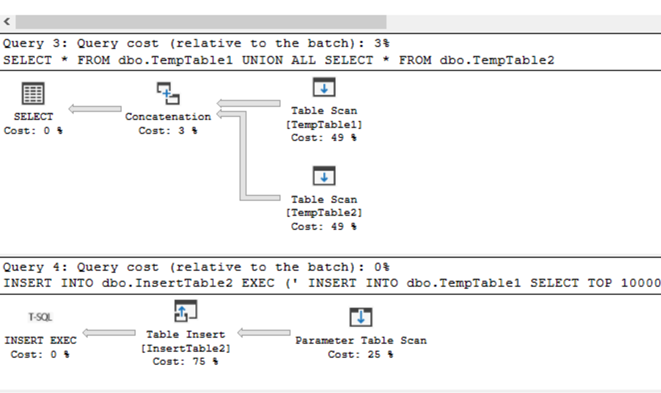
Execution plan

 

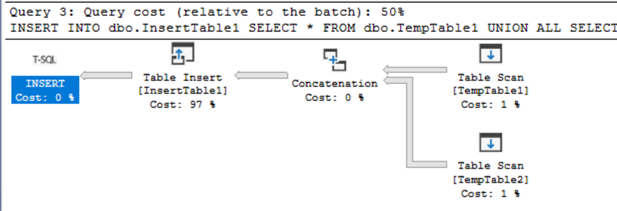
The difference in execution plan is as follow. With INSERT – EXEC you get two statements. The one for the result-set of EXEC and the second one for inserting the data.

Transaction log

Another perspective is the transaction scope behaviour. Let’s get data from transaction_log event to temporary tables first.

SELECT     CAST (EVENT_data AS XML).value('(/event/data[@name="log_record_size"])[1]','INT') logsize,
CAST (EVENT_data AS XML).value('(/event/@timestamp)[1]','datetime2') timestamp,
CAST (EVENT_data AS XML).value('(/event/data[@name="transaction_start_time"])[1]','datetime2') date_time,
CAST (EVENT_data AS XML).value('(/event/data[@name="database_id"])[1]','INT')    database_id,
CAST (EVENT_data AS XML).value('(/event/data[@name="transaction_id"])[1]','INT')    transaction_id,
CAST (EVENT_data AS XML).value('(/event/action[@name="sql_text"])[1]','VARCHAR(1000)')    sql_text ,
CAST (EVENT_data AS XML).value('(/event/data[@name="operation"])[1]','VARCHAR(1000)')    operation
INTO #t1
FROM sys.fn_xe_file_target_read_file('C:\outputfile\outputfile1*.xel', 'C:\outputfile\outputfile1*.xem', null, null)
WHERE object_name = 'transaction_log' ;

SELECT CAST (EVENT_data AS XML).value('(/event/data[@name="log_record_size"])[1]','INT') logsize,
CAST (EVENT_data AS XML).value('(/event/@timestamp)[1]','datetime2') timestamp,
CAST (EVENT_data AS XML).value('(/event/data[@name="transaction_start_time"])[1]','datetime2') date_time,
CAST (EVENT_data AS XML).value('(/event/data[@name="database_id"])[1]','INT')    database_id,
CAST (EVENT_data AS XML).value('(/event/data[@name="transaction_id"])[1]','INT')    transaction_id,
CAST (EVENT_data AS XML).value('(/event/action[@name="sql_text"])[1]','VARCHAR(1000)')    sql_text ,
CAST (EVENT_data AS XML).value('(/event/data[@name="operation"])[1]','VARCHAR(1000)')    operation
INTO #t2
FROM sys.fn_xe_file_target_read_file('C:\outputfile\outputfile2*.xel', 'C:\outputfile\outputfile2*.xem', null, null)
WHERE object_name = 'transaction_log' 
;

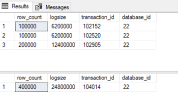
 Comparing following query outputs, we can see that insert-exec is scoped by one transaction against multiple individual transactions with normal insert.

SELECT COUNT(1) row_count,SUM(logsize) logsize,transaction_id,database_id FROM #t1 WHERE operation = '2LOP_INSERT_ROWS' GROUP BY transaction_id ,database_id

SELECT COUNT(1) row_count,SUM(logsize) logsize,transaction_id,database_id FROM #t2 WHERE operation = '2LOP_INSERT_ROWS' GROUP BY transaction_id, database_id

Transaction scope

In case of INSERT-EXEC statement it should rollback all insert statements inside of EXEC statement when error occurs, because INSERT – EXEC is scoped by one transaction. In case of individual transactions in stored procedure, each insert is taken like separate transaction, so rollbacked will be insert resulting with error. Let’s try:

Change type of inserting value to INT column in second insert.

INSERT INTO dbo.TempTable2
SELECT TOP 100000 REPLICATE('a',10 ) REPLICATE('a',10 ) a
FROM sys.objects a
JOIN sys.objects b ON 1=1

Run testing queries again. As you can see in case of INSERT-EXEC statement there are no rows inserted in tables since rollback appears.

Conclusion:

While INSERT-EXEC statement still takes place in some scenarios, you should be aware of mentioned circumstances.

NOTICE: I would like to check that transaction log of temporary database was filled with connection to the worktable created by INSERT-EXEC statement. But I cannot see any insert lop insert operation trough extended events in temporary database. I just see extent allocation

SELECT * FROM #t2 WHERE database_id = 2

 If you have any idea whether worktables are logged and it is possible to trace them, please write a comment.